MOC (Multi-Objective Counterfactual Explanations) for Regression Tasks
Source:R/MOCRegr.R
MOCRegr.RdMOC (Dandl et. al 2020) solves a multi-objective optimization problem to find counterfactuals. The four objectives to minimize are:
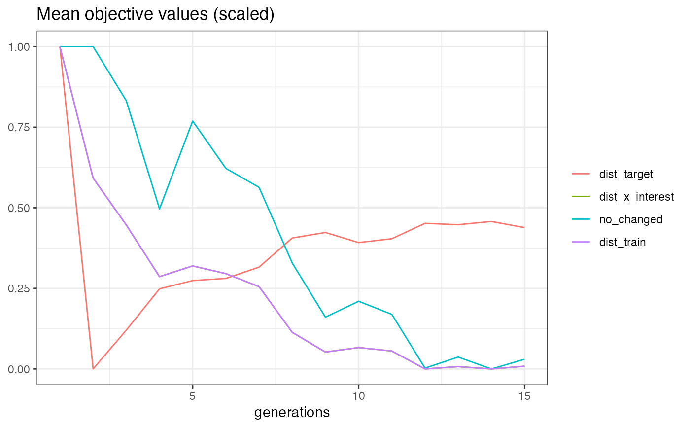
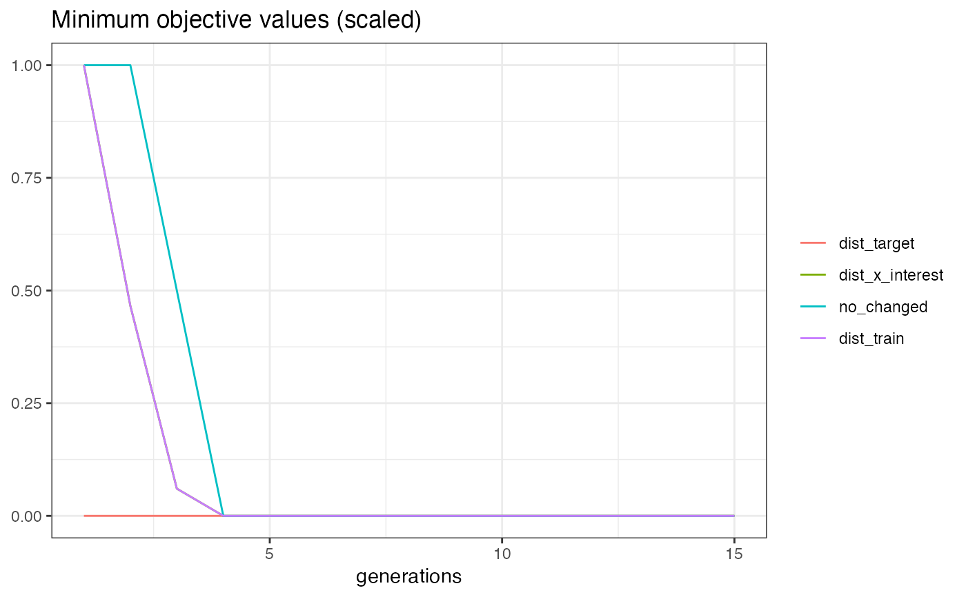
dist_target: Distance todesired_prob(classification tasks) ordesired_prob(regression tasks).dist_x_interest: Dissimilarity tox_interestmeasured by Gower's dissimilarity measure (Gower 1971).no_changed: Number of feature changes.dist_train: (Weighted) sum of dissimilarities to theknearest data points inpredictor$data$X.
For optimization, it uses the NSGA II algorithm (Deb et. al 2002) with mixed integer evolutionary strategies (Li et al. 2013) and some tailored adjustments for the counterfactual search (Dandl et al. 2020). Default values for the hyperparameters are based on Dandl et al. 2020.
Details
Several population initialization strategies are available:
random: Feature values of new individuals are sampled from the feature value ranges inpredictor$data$X. Some features values are randomly reset to their initial value inx_interest.sd: Likerandom, except that the sample ranges of numerical features are limited to one standard deviation from their initial value inx_interest.icecurve: As inrandom, feature values are sampled from the feature value ranges inpredictor$data$X. Then, however, features are reset with probabilities relative to their importance: the higher the importance of a feature, the higher the probability that its values differ from its value inx_interest. The feature importance is measured using ICE curves (Goldstein et al. 2015).traindata: Contrary to the other strategies, feature values are drawn from (non-dominated) data points inpredictor$data$X; if not enough non-dominated data points are available, remaining individuals are initialized by random sampling. Subsequently, some features values are randomly reset to their initial value inx_interest(as forrandom).
If use_conditional_mutator is set to TRUE, a conditional mutator samples
feature values from the conditional distribution given the other feature values
with the help of transformation trees (Hothorn and Zeileis 2017).
For details see Dandl et al. 2020.
References
Dandl, S., Molnar, C., Binder, M., & Bischl, B. (2020). "Multi-Objective Counterfactual Explanations". In: Parallel Problem Solving from Nature – PPSN XVI, edited by Thomas Bäck, Mike Preuss, André Deutz, Hao Wang, Carola Doerr, Michael Emmerich, and Heike Trautmann, 448–469, Cham, Springer International Publishing, doi:10.1007/978-3-030-58112-1_31 .
Deb, K., Pratap, A., Agarwal, S., & Meyarivan, T. A. M. T. (2002). "A Fast and Elitist Multiobjective Genetic Algorithm: NSGA-II". IEEE Transactions on Evolutionary Computation, 6(2), 182-197.
Goldstein, A., Kapelner, A., Bleich, J., & Pitkin, E. (2015). "Peeking Inside the Black Box: Visualizing Statistical Learning with Plots of Individual Conditional Expectation". Journal of Computational and Graphical Statistics 24 (1): 44–65. doi:10.1080/10618600.2014.907095 .
Gower, J. C. (1971). "A General Coefficient of Similarity and Some of its Properties". Biometrics, 27, 623–637.
Hothorn, T., & Zeileis, A. (2017), "Transformation Forests". Technical Report, arXiv 1701.02110.
Li, Rui, L., Emmerich, M. T. M., Eggermont, J. Bäck, T., Schütz, M., Dijkstra, J., & Reiber, J. H. C. (2013). "Mixed Integer Evolution Strategies for Parameter Optimization." Evolutionary Computation 21 (1): 29–64. doi:10.1162/EVCO_a_00059 .
Super classes
counterfactuals::CounterfactualMethod -> counterfactuals::CounterfactualMethodRegr -> MOCRegr
Active bindings
optimizer(OptimInstanceBatchMultiCrit)
The object used for optimization.
Methods
Method new()
Create a new MOCRegr object.
Usage
MOCRegr$new(
  predictor,
  epsilon = NULL,
  fixed_features = NULL,
  max_changed = NULL,
  mu = 20L,
  termination_crit = "gens",
  n_generations = 175L,
  p_rec = 0.71,
  p_rec_gen = 0.62,
  p_mut = 0.73,
  p_mut_gen = 0.5,
  p_mut_use_orig = 0.4,
  k = 1L,
  weights = NULL,
  lower = NULL,
  upper = NULL,
  init_strategy = "icecurve",
  use_conditional_mutator = FALSE,
  quiet = FALSE,
  distance_function = "gower"
)
Arguments
predictor(Predictor)
The object (created withiml::Predictor$new()) holding the machine learning model and the data.epsilon(
numeric(1)|NULL)
If notNULL, candidates whose prediction is farther away from the intervaldesired_outcomethanepsilonare penalized.NULL(default) means no penalization.fixed_features(
character()|NULL)
Names of features that are not allowed to be changed.NULL(default) allows all features to be changed.max_changed(
integerish(1)|NULL)
Maximum number of feature changes.NULL(default) allows any number of changes.mu(
integerish(1))
The population size. Default is20L.termination_crit(
character(1)|NULL)
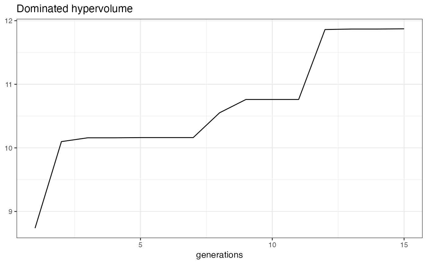
Termination criterion, currently, two criterions are implemented: "gens" (default), which stops aftern_generationsgenerations, and "genstag", which stops after the hypervolume did not improve forn_generationsgenerations (the total number of generations is limited to 500).n_generations(
integerish(1))
The number of generations. Default is175L.p_rec(
numeric(1))
Probability with which an individual is selected for recombination. Default is0.71.p_rec_gen(
numeric(1))
Probability with which a feature/gene is selected for recombination. Default is0.62.p_mut(
numeric(1))
Probability with which an individual is selected for mutation. Default is0.73.p_mut_gen(
numeric(1))
Probability with which a feature/gene is selected for mutation. Default is0.5.p_mut_use_orig(
numeric(1))
Probability with which a feature/gene is reset to its original value inx_interestafter mutation. Default is0.4.k(
integerish(1))
The number of data points to use for the forth objective. Default is1L.weights(
numeric(1) | numeric(k)|NULL)
The weights used to compute the weighted sum of dissimilarities for the forth objective. It is either a single value or a vector of lengthk. If it has lengthk, the i-th element specifies the weight of the i-th closest data point. The values should sum up to1.NULL(default) means all data points are weighted equally.lower(
numeric()|NULL)
Vector of minimum values for numeric features. IfNULL(default), the element for each numeric feature inloweris taken as its minimum value inpredictor$data$X. If notNULL, it should be named with the corresponding feature names.upper(
numeric()|NULL)
Vector of maximum values for numeric features. IfNULL(default), the element for each numeric feature inupperis taken as its maximum value inpredictor$data$X. If notNULL, it should be named with the corresponding feature names.init_strategy(
character(1))
The population initialization strategy. Can beicecurve(default),random,sdortraindata. For more information, see theDetailssection.use_conditional_mutator(
logical(1))
Should a conditional mutator be used? The conditional mutator generates plausible feature values based on the values of the other feature. Default isFALSE.quiet(
logical(1))
Should information about the optimization status be hidden? Default isFALSE.distance_function(
function()|'gower'|'gower_c')
The distance function to be used in the second and fourth objective. Either the name of an already implemented distance function ('gower' or 'gower_c') or a function. If set to 'gower' (default), then Gower's distance (Gower 1971) is used; if set to 'gower_c', a C-based more efficient version of Gower's distance is used. A function must have three argumentsx,y, anddataand should return adoublematrix withnrow(x)rows and maximumnrow(y)columns.
Method plot_statistics()
Plots the evolution of the mean and minimum objective values together with the dominated hypervolume over the generations. All values for a generation are computed based on all non-dominated individuals that emerged until that generation.
Method plot_search()
Visualizes two selected objective values of all emerged individuals in a scatter plot.
Usage
MOCRegr$plot_search(objectives = c("dist_target", "dist_x_interest"))Examples
if (require("randomForest")) {
# Train a model
rf = randomForest(mpg ~ ., data = mtcars)
# Create a predictor object
predictor = iml::Predictor$new(rf)
# Find counterfactuals for x_interest
# \donttest{
moc_regr = MOCRegr$new(predictor, n_generations = 15L, quiet = TRUE)
cfactuals = moc_regr$find_counterfactuals(x_interest = mtcars[1L, ], desired_outcome = c(22, 26))
# Print the counterfactuals
cfactuals$data
# Plot evolution of hypervolume and mean and minimum objective values
moc_regr$plot_statistics()
# }
}
#> `x_interest` was removed from results.
#> [[1]]
 #>
#> [[2]]
#>
#> [[2]]
 #>
#> [[3]]
#>
#> [[3]]
 #>
#>